I set out to build a BERT like encoder from scratch this year. But that's not what happened. Instead I spent months stumbling over my inexperience, hitting walls, abandoning assumptions, and ultimately leaning on pretrained weights just to get off the ground. This is that retrospective—every wrong turn, every silent bug, and the hard-won lessons that came from building something I barely understood when I started.
The Vision and the Naivety
My original goal was ambitious: write an encoder from the ground up, train it on biblical text using Masked Language Modeling, and build a hybrid search for the New Testament. I wanted to understand embeddings at the deepest level, and this project was the proving ground. With the original BERT paper in hand I set out to reproduce their success on a much smaller corpus—and I was wildly underestimating what lay ahead. Nothing about this would come together quickly, and early wins like moving from SGD to the Adam optimizer only revealed the volume of problems hiding underneath.
What followed was months of exploration, discovery, dead ends, and hard-won lessons. Like all of my adventures, the mistakes were the most interesting part of the story.
The First Wall: Padding Masks
The biggest trap I fell into early on was assuming the compiler would find bugs for me. I jumped straight into training runs with complex architectures, convinced that more layers meant better results. I should have started by trying to memorize 100 tokens over 10 epochs to validate simple base assumptions.
For a while I did see training loss improve, but validation loss was inconsistent. I didn't train long enough to see the plateau, which gave me a false impression that my attention implementation was working. Eventually I found that learning a single verse was possible, but when I tried to learn 10 verses—with an overfitting, repetitive dataset just to prove it could work—everything fell apart.
That's when I pulled back to inspect the math behind each component individually.
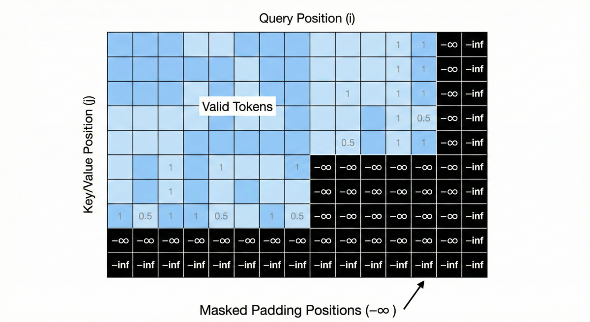
I used IO.inspect to print out the vectors for a shorter verse. The last 20 tokens were clearly padding IDs. I traced query, key, and value projections and realized I wasn't excluding padding positions from attention.
The model was learning from padding. That single masking error was hiding behind what looked like architecture problems and sent me down more than a few dead ends.
The fix was an additive mask that sets padding positions to negative infinity before softmax, effectively zeroing them out:
    defn self_attention(input, w_query, w_key, w_value, w_out, attention_mask) do
      # ... projection code ...

      attention_scores = Nx.dot(q, [3], [0, 1], k, [3], [0, 1])
      scaling_divisor = Nx.sqrt(head_dim)
      scaled_attention_scores = Nx.divide(attention_scores, scaling_divisor)

      # The fix: -1.0e8 makes padding positions effectively zero after softmax
      additive_mask = Nx.select(attention_mask, 0.0, -1.0e8)
      masked_scores = Nx.add(scaled_attention_scores, additive_mask)

      attention_weights = softmax(masked_scores)
      # ... rest of attention ...
    end
Once I properly implemented padding masks, performance jumped dramatically. The learning: there are no shortcuts—you need to verify your math step-by-step on a tiny dataset before scaling up.
The Second Wall: Gradient Chaos
For the longest time, I never computed or printed my gradients to evaluate them. I was hypnotized by my training and validation loss curves, completely ignoring the underlying mathematics.
The symptom was that validation loss didn't have a nice curve. It would improve, then jump around, never settling into the steady descent I expected. So much code had been written at this point, and much of it wasn't properly validated.
I spent some time digging into the Polaris library so I could compute gradients, and with that additional information I was finally able to see the problem: gradient explosion.
Before epoch 6 or 8, the gradient norm would be something like 12. But as training continued I would see 18, then 20, then 33—and it never came down. I consulted with Gemini about this pattern, and you might say I took the LLM's word as gospel: this was a bad signal indicating erratic learning.
From here, I read about gradient clipping and discovered how the original BERT team clipped at 1.0. The fix was straightforward with Polaris:
    {init_fn, update_fn} =
      Polaris.Updates.clip_by_global_norm(max_norm: 1.0)
      |> Polaris.Updates.scale_by_adam()
      |> Polaris.Updates.add_decayed_weights(decay: 0.01)
      |> Polaris.Updates.scale_by_schedule(schedule_fn)

    init_optimizer_state = init_fn.(initial_params)
This single change transformed my erratic training into steady, predictable progress. The learning: your gradients are telling you a story. Listen to them.
The Third Wall: Memory Leaks
As I started to scale up my encoder, my RTX 4090 ran out of vRAM by epoch 8 or 10. I moved to the cloud with RunPod using my runpod-cuda12 setup, and even an 80GB H100 failed after 16 hours. That was the clue: this wasn't a hardware limit—it was a leak.
The issue was simple. I had Nx.backend_deallocate calls, but not in the innermost loop. The first batch of each epoch accumulated without release. Memory grew every epoch until the run collapsed around epoch 8-10.
After moving deallocation into the inner loop, I was able to cut my cloud spending and go back to training at home with just one more trick: I cracked open the Nx types.ex file in my deps directory and changed the default float from f32 to bf16. This is still a direct hack—as of this writing, the configuration doesn't yet exist in Nx—but it allowed me to run without compromise in terms of layers, dimensionality, or attention heads.
The Architecture Shift: Pre-Layer Normalization
While training loss was improving, validation loss wasn't moving with my bigger dataset. After fixing the padding mask issue, I set my sights on this problem along with trying to dial in the number of layers and attention heads.
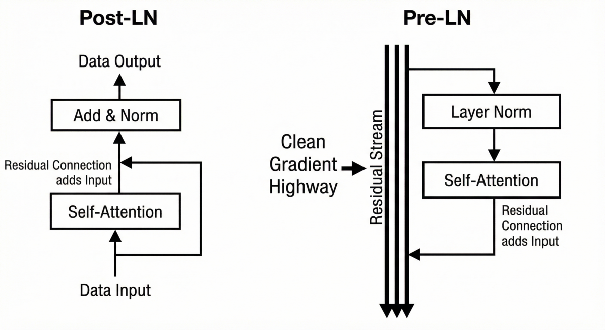
I originally had post-layer normalization—the pattern from the original BERT paper where you normalize after the residual connection. After some chatting with Claude about my architecture, it recommended I try pre-layer normalization instead.
The difference is subtle but important. Post-LN (original BERT):
    # Post-LN: normalize AFTER residual add
    attn_out = self_attention(x, ...)
    add = residual_connection(x, attn_out)
    norm = layer_norm(add)
Pre-LN (what I switched to):
    # Pre-LN: normalize BEFORE sublayer
    norm_attn = layer_norm(x)
    attn_out = self_attention(norm_attn, ...)
    add = residual_connection(x, attn_out)
Why does this matter? In post-LN, gradients must flow through normalization after the residual add. As you stack layers, 12 in my case, that compounding effect can either explode or vanish before it reaches early layers.
Pre-LN keeps the residual path clean. The gradient can flow directly through x + sublayer_output without passing through normalization, while attention and FFN paths still get normalized.
The original BERT team used post-LN with 12 layers, but they also had massive compute, huge datasets, and the ability to tune endlessly. With fewer than 500,000 examples, I needed stability. Pre-LN gave me predictable gradients and a much more forgiving learning rate.
The Recipe Ceiling
After countless training runs and months of tuning the encoder, validation loss was stuck around 1.6. I'd tried everything I could think of: adjusting dropout rates, tweaking learning rates, adding layers or attention head dimensions, increasing weight decay. Nothing broke through the floor. I was convinced I'd hit a data ceiling—that 400,000 training examples simply weren't enough.
Then I pulled in a fresh pair of eyes for a detailed code review, stepping through each component of the training loop. Within hours, two foundational bugs surfaced that had been compounding since my first training run.
First, my dropout implementation was fundamentally wrong. I used a normal distribution for the mask, which quietly dropped far more activations than intended. The model was training under a much harsher regularizer than I thought, and the surviving activations were scaled as if nothing was wrong. It was a silent, destructive bug that made everything look like a data problem.
The fix was textbook dropout—switch to a uniform distribution with a proper Bernoulli mask:
    defn dropout(input, key, training) do
      if training do
        mask_shape = Nx.shape(input)
        random_vals = Nx.Random.uniform_split(key, 0.0, 1.0, shape: mask_shape)
        keep_prob = Nx.subtract(1.0, @dropout_rate)
        keep_mask = Nx.less(random_vals, keep_prob)
        scale_factor = Nx.divide(1.0, keep_prob)
        input |> Nx.multiply(keep_mask) |> Nx.multiply(scale_factor)
      else
        input
      end
    end
Second, my masked language modeling targets were static. Masking happened once during preprocessing, and every epoch saw the exact same masked positions with the same targets. The model could memorize "token 47 is always masked in example 312" rather than learning general language structure. With static masks, my 400,000 examples were effectively a much smaller dataset because the supervised signal never varied.
The fix was to separate tokenization from masking—tokenize once during preprocessing, then apply masks dynamically per batch at training time. This mirrors standard BERT practice and means the model sees different masked positions every epoch, turning each example into many variants of itself.
The results were immediate and dramatic:
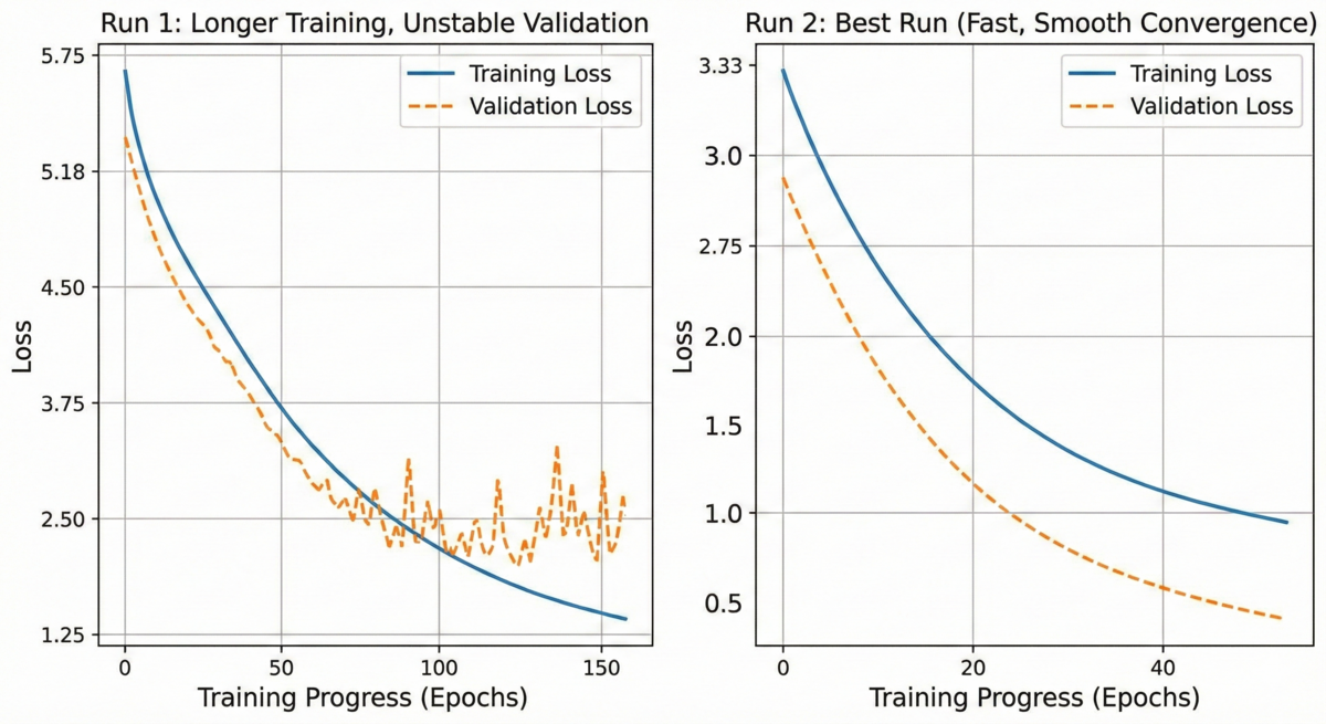
By epoch 8, Run 8 already beat the best validation loss across all seven previous runs. By epoch 12, it reached 1.124—a 29% improvement over a ceiling I'd spent months trying to break through. The overfitting I'd been fighting wasn't a data ceiling at all. It was a recipe ceiling.
The Missing Projection: Weight Tying
With my loss curves looking better than ever, I thought I was finally at the end of my journey. Unfortunately, my evals showed a lack of depth because of another critical detail I skipped over early on.
At some point I came to grips with the reality that I couldn't train weights from scratch like the team behind BERT—I didn't have a dataset anywhere near 3 billion tokens. So instead I gave myself a jump start by borrowing the initial weights from all 12 layers of BERT-base. The trouble was that I forgot to include the vocab projection weights, so the final MLM head failed to project my learned geometry into the proper vocabulary.
My evaluation suite told the whole story. The encoder clearly understood theology—75% accuracy on contrastive tests—but couldn't predict the right vocabulary words at masked positions:
    DOC_001: expected=grace    got=[your(0.37), their(0.20), per(0.10), rep(0.05), ab(0.03)]
    DOC_010: expected=image    got=[the(0.98), and(0.01), ##the(0.00), ##d(0.00), ##th(0.00)]
    DOC_025: expected=kingdom  got=[father(0.999), ##otte(0.00), beg(0.00), ##k(0.00), ab(0.00)]
The model was predicting function words, subword fragments, and punctuation instead of theological terms. Even at k=50, not a single doctrinal target appeared. The encoder's internal representations were strong, but the output projection to vocabulary was completely broken because I had initialized my MLM output weights randomly and never tied them to the embedding matrix.
In a BERT encoder, two matrices deal with the vocabulary. The embedding matrix maps token IDs to 768-dimensional vectors at the input. The output projection maps those 768-dimensional hidden states back to vocabulary logits at masked positions. These two matrices perform inverse operations—one goes from vocabulary to hidden space, the other goes back. Weight tying makes this relationship explicit by using the same matrix for both:
    # Without weight tying: two independent matrices
    logits = Nx.dot(hidden_states, out_w) |> Nx.add(out_b)

    # With weight tying: one matrix, transposed for output
    logits = Nx.dot(hidden_states, Nx.transpose(embeddings)) |> Nx.add(out_b)
The out_w parameter disappears entirely. The embedding matrix serves double duty, and every gradient that updates the embedding for "grace" simultaneously updates how the model predicts "grace" at masked positions. Without weight tying, I was asking a random matrix to decode a learned representation space—hoping that 768 x 30,522 parameters would independently converge to match the encoder's geometry. They never did.
This also cut ~23 million trainable parameters, which meant less memory and smaller optimizer state. More importantly, it eliminated a failure mode: if the encoder knows what "grace" means, it could now predict "grace" at a masked position, because the same vector represents both.
Aligning for Search: Contrastive Training
With a solid MLM training behind me, I set my sights on the work ahead to align this encoder for search tasks. MLM taught the model to understand tokens in context—"fill in the blank"—but search requires something different. I needed similar meanings to cluster together in the embedding space so that a query and a relevant verse would land near each other.
To get there, I put together a dataset of paired verses drawn from different Bible translations. The same verse in the NLT and NIV is a natural positive pair—same meaning, different wording. I then took the final MLM weights and trained with a contrastive loss function that would pull matching pairs closer together while pushing everything else apart.
The approach works by encoding both sides of a pair through the same encoder, mean-pooling the token outputs into a single sentence vector (with pad masking so padding doesn't count), and then L2-normalizing so cosine similarity becomes a simple dot product. For a batch of 64 pairs, this builds a 64x64 similarity matrix where the diagonal entries are the correct matches and everything off-diagonal is an implicit negative:
While this was the simplest post-training and least error prone step throughout, it still came with some valuable learnings. The one that stuck with me is the key difference in the loss functions. In this training run the model is no longer predicting individual tokens. It's answering: "which sentence out of these 64 (batch size) is the true partner?"
This fine-tuning step took the encoder from understanding words in context to understanding that two differently worded verses about the same concept should live in the same neighborhood of embedding space.
The Last Mile: Query-to-Verse Alignment
After contrastive training, I had an encoder that grouped similar verses together but there was still a gap between how the encoder organized scripture and how a person actually searches. People usually search with short phrases or even questions shaped by their own vocabulary and experience with other software, which often doesn't overlap with the biblical text at all.
To close that gap, I generated a dataset of 1,400 high-quality query-to-verse mappings. Each pair linked a natural search phrase to the verse it was really asking about. For example, "assurance of salvation" mapped to Romans 8:1—"there is therefore now no condemnation for those who are in Christ Jesus." The verse never mentions the word "salvation," but it speaks directly to that theology.
The training used the same contrastive loss as before, but with a fundamentally different dataset. Instead of teaching the encoder that two translations of the same verse should be neighbors, I was teaching it that a human search query and its best answer should be neighbors. This bent the geometry one final time —pulling the embedding space toward how people actually look for scripture, not just how scripture relates to itself.
This was the smallest dataset of the three training phases, but arguably the most targeted. The 1,400 pairs acted as precise instructions: when someone asks about "forgiveness after failure," the encoder should point toward the prodigal son, not just verses that happen to contain the word "forgiveness." Quality mattered far more than quantity here, requiring loads of synthetic data engineering and genuine theological care to validate the mappings before training.
The Missing Baseline: BM25
If I had to do it all over again, I would have started with BM25 as my baseline from day one—not bolted it on toward the end as an afterthought. Keyword search isn't just a fallback. It's a genuinely powerful complement to semantic search, and understanding why made the final hybrid experience far better than either approach alone.
BM25 and semantic search fail in complementary ways. BM25 excels when the user's words overlap with the text—exact phrases, proper nouns, specific references. The encoder excels when they don't: thematic queries like "assurance of salvation" or "fruit of the spirit" surface verses that speak to the concept without containing the exact keywords. The keyword signal anchors results for literal queries while the encoder lifts thematic results that pure text matching would miss.
The challenge with combining them is that their scores live on completely different scales, so a naive weighted sum is notoriously difficult to tune. Reciprocal Rank Fusion sidesteps the problem entirely by ignoring raw scores and working only with rank positions—a document ranked highly by both rises to the top without any normalization at all.
Starting with BM25 as the baseline would have given me a strong search experience much earlier and a clearer benchmark for measuring what the encoder actually added.
The Data Reckoning
More than anything, I spent months building, curating, and tuning my dataset. I knew I couldn't achieve the same size and diversity the original BERT team had, but I was pleasantly surprised with what I could accomplish with just under 500,000 unique training examples.
The trouble was I made several mistakes that cost me significant time:
False diversity. I wanted a diverse set of Bible text and found myself using different translations—NLT, NIV, ESV, NET. This seemed like a good idea, but I didn't actually look at the dataset closely. While subtle differences exist between translations, they share similar tokens and themes. They aren't radically different. I later learned I should have included genuinely different text like Mere Christianity, rich theological writing that isn't the original Bible text.
Quote noise. Biblical text has a lot of quotation marks, and I found this was distracting to the masked token prediction with my simplistic encoder. The model was learning patterns around quote boundaries rather than semantic meaning.
Lazy first pass. While I expanded to books over time, I didn't do my best work on the first pass. A lot of that text data was less than ideal until I circled back to do real cleaning—which only happened by actually reading the text in those contextualized chunks.
If I had to synthesize what I would do differently, it comes down to this: look at the data more. I underestimated the time involved in data work, which has become a recurring theme throughout my machine learning journey.
The Invisible Bugs
Looking back across every wall I hit, the pattern was always the same: something that appeared to work was silently wrong.
Padding masks didn't throw errors—attention just quietly attended to nonsense. Dropout didn't crash—it just dropped 56% of activations instead of 16%. Static masking didn't fail—it let the model memorize targets instead of learning language. The output projection didn't break—it just never converged to match the encoder's geometry. In every case, training loss went down and nothing in the logs said something was broken.
The most dangerous bugs in machine learning are the ones that look like they're working. If you're building a model from scratch, the single most valuable habit I can offer is this: validate every component in isolation on a tiny dataset before scaling up. Print the vectors. Inspect the gradients. Check that your dropout rate actually drops what you think it drops. And when you hit what looks like a ceiling, get a fresh pair of eyes on your code before you assume it's a data problem.
You can find the source code on github.
